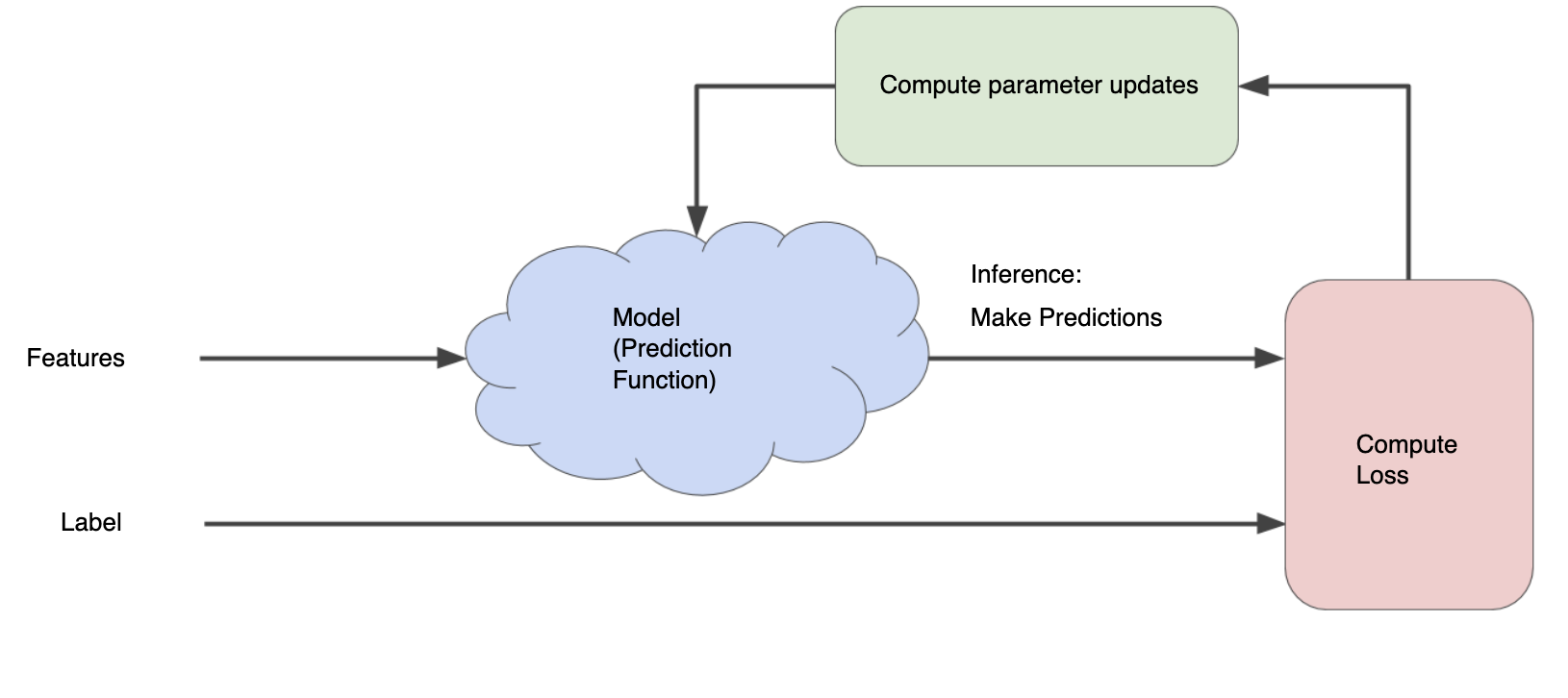
Intro to Supervised Machine Learning

Dr. Will Horne

What is Supervised Machine Learning

• A wide range of models, ranging from naive bayes and logit to support vector machines and random forests

• All share the same work flow: Train, Test, Validate!

• Goal: Train models on labeled data that preform well on out-of-sample, new data

Terminology (1)

Our data have labels. This is the target of our prediction. Analogous to our Y in a regression.

Our data also have features. This is the X terms in a regression.

For example, our label might be whether the speaker was for or against a policy (1 or 0). The features might be the words spoken, or might be information about the speaker (race, age, gender, partyID).

Data Structure

Feat 1: Age	Feat 2: Gender	Feat 3: PartyID	Feat4: Text	Label:
61	F	D	I support this bill…	1
55	M	D	I respectfully…	0
42	M	R	I oppose this plan…	0
73	F	R	This radical left…	0
46	M	D	I rise in favor of…	1

Terminology (2)

Training: We train the model by showing it labeled data. The model learns the relationships between the features and data.

Hyperparamters: Parameters of the model set by users. We can adjust things like learning rate, batch size, number of epochs (training length) and other method specific hyperparamters.

Inference in machine learning comes when we apply our trained model to new, unlabeled data.

About labeled data

Sometimes, you will be lucky and you will have labels (votes, partisanship, etc) and you simply want a model that does well at prediction.

Frequently, you will have to label your own data. Transparent coding rules are key, and if possible documents should be labeled by multiple coders allowing for measures of inter-coder reliability.

Labeling data is expensive and time consuming. I’ve been overseeing a project for a year now, and we are still labeling! LLMs may and embeddings may be able to help for some labeling tasks.

OLS

\[ Y = X\beta + \epsilon \]

We all know and love(?) OLS. It’s BLUE !

How do we get our vector \(\beta\) ?

Can we think about OLS as a machine learning model?

OLS as a Machine Learning Model

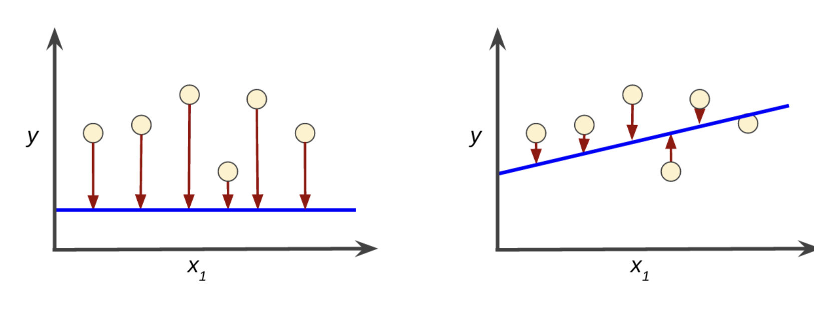
How do we know we have a good line? We need a loss function

The OLS Loss Function

In OLS, our loss function is squared loss or \(L_{2}\) loss. This gives us an objective function to minimize, which is mean squared error:

\[ MSE = \frac{1}{N} \sum_{(x,y)\in D} (y - \text{prediction(x)})^{2} \]

Where D is the data, and N is the number of examples in D. Prediction(x) can also be written as \(\widehat{y}|x\)

Now what?

Ok…now we have a loss function that we want to minimize. Now What???

Step 1: Draw a random line through the data (this is the initialization step)

Step 2: ????

Step 3: Profit

An Iterative Approach

Step 1: Draw a random line through the data (this is the initialization step)

Step 2: Calculate the loss

Step 3: Draw a (slightly) different line

Step 4: Calculate the loss.

Step 5: Repeat until the model converges (the loss stops changing)

Graphically

A more principled approach

We want to minimize our loss function:

\[ MSE = \frac{1}{N} \sum (\widehat{Y} - Y)^{2} \]

and our equation is \[ \widehat{Y} = \beta_{0} + \beta_{1} X\] (ignoring the error term).

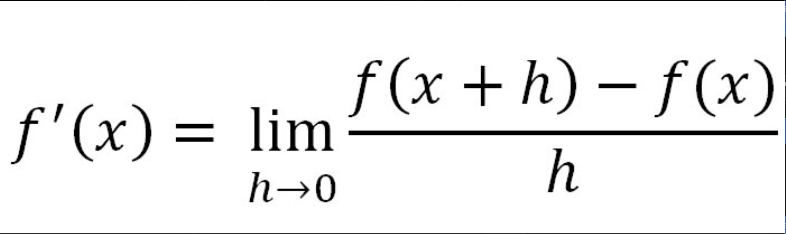
Wait - How do we min(or max)imize something?

What the heck is a derivative?

NO!!!

Yes!!!

This type of derivative will never destroy the global economy!

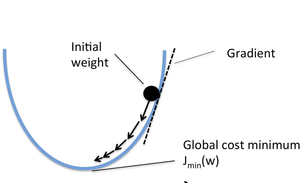
Gradient Descent

Derivative Rules

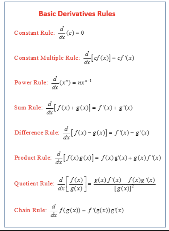
What is the derivative of our loss function wrt \(\beta_{0}\) and wrt \(\beta_{1}\)?

Take the Derivative of the Loss Function

\[ \frac{\partial L}{\partial \beta{i}} = \frac{2}{N} \sum(\widehat{Y} - Y) * \frac{\partial \widehat{Y}}{\partial \beta_{i}} \]

Updating

Intuitively - what happens to the loss if we nudge \(\beta\) a little bit in one direction

Formally, that little bit is defined by \(\alpha\) (the learning rate) and the gradients/derivatives are the sums of the errors. Meaning:

\[ \beta_{0}^{k+1} = \beta_{0}^{K} - [\alpha\sum(\widehat{Y} - Y)] \]

\[ \beta_{1}^{k+1} = \beta_{1}^{K} - [\alpha \sum(\widehat{Y} - Y)X] \]

A quick aside on learning rate

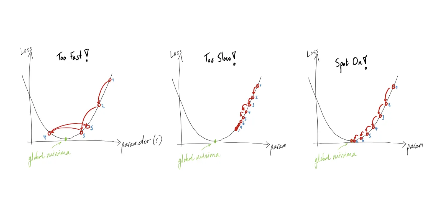
If we set the loss rate too low, it will take forever to converge. What happens if we set it too high?

Congratulations!

This is gradient descent. Much of machine learning (esp deep learning) is built on it! You are now a machine learning engineer.

Recap

Step 1: Draw a random line through the data (this is the initialization step)

Step 2: Calculate the derivative off the loss wrt the weights (aka coefficients)

Step 3: Nudge the model slightly in direction of the derivative, as determined by \(\alpha\)

Step 4: Repeat until the model converges (the loss stops changing)

Classification

Most text as data SML problems are classification problems, although most of the methods can also be used for regression.

For classification, we predict labels for categorical data.

Is the speaker a Democrat or Republican?

Is the sentiment positive or negative?

Classification has a different set of metrics than regression.

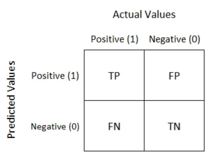
Classification Terminology

True Positive: \(\widehat{y_{i}} = 1\), \(y_{i} = 1\)

False Positive: \(\widehat{y_{i}} = 1\), \(y_{i} = 0\)

True Negative: \(\widehat{y_{i}} = 0\), \(y_{i} = 0\)

False Negative: \(\widehat{y_{i}} = 0\), \(y_{i} = 1\)

Confusion Matrices

Confusion Matrices can be extended

Alternatively

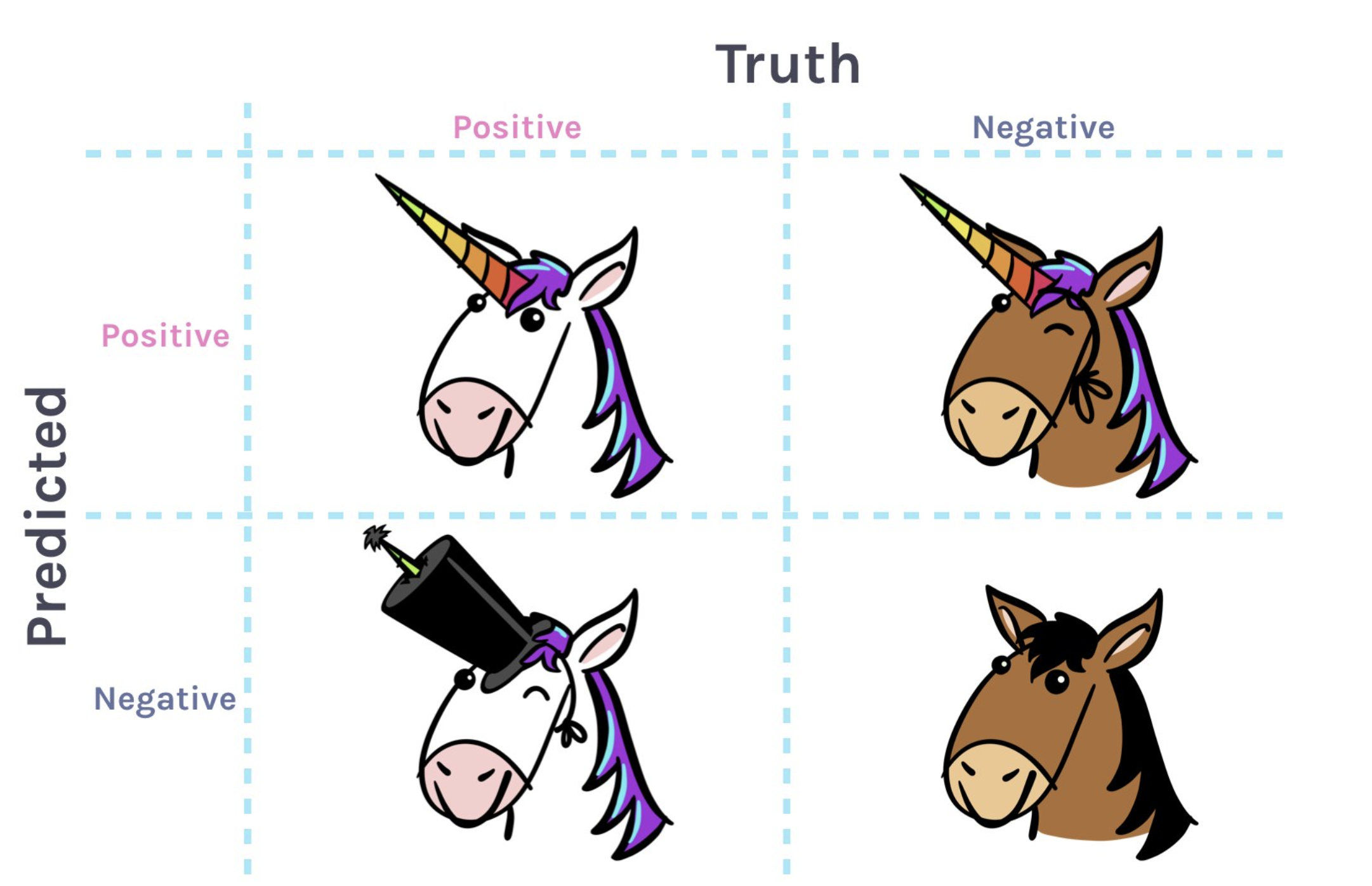
Image credit Allison Horst

Metrics

Metric	Formula
Accuracy:	\(\frac{TP + TN}{TP + TN + FP + FN}\)
Precision:	\(\frac{TP}{TP + FP}\)
Recall:	\(\frac{TP}{TP + FN}\)
F1 Score:	\(2 * \frac{\text{precision}*\text{recall}}{\text{precision} + \text{recall}}\)

ROC CURVE

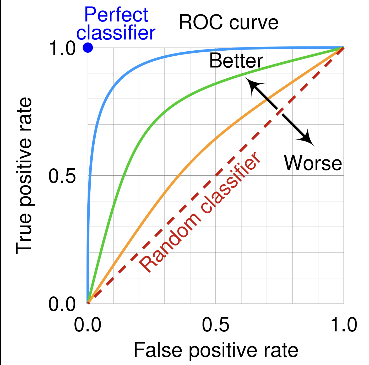
Intution: How the model performs at different classification thresholds.

TPR = Recall (TP / TP + FN)

FPR = (FP / TN + TP)

Unbalanced Data

A getting into Harvard classifier could trivially have great accuracy!

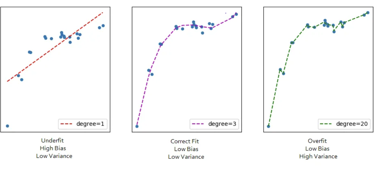
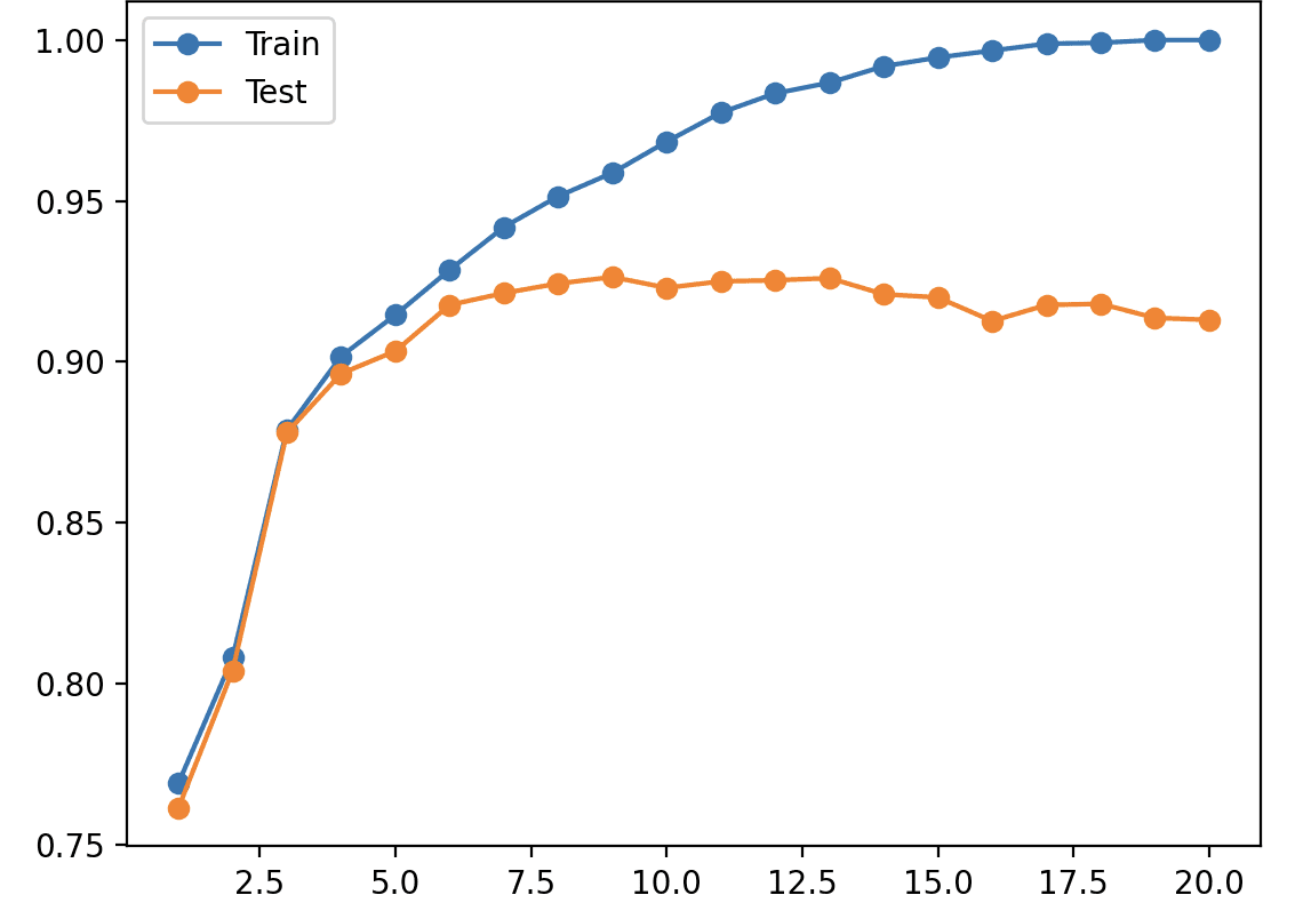
Overfitting is a problem!

We can train our models to be incredibly accurate on the training data.

But…we don’t care how well a model does on training set.

A supervised machine learning model is measured by how well it fits unseen data

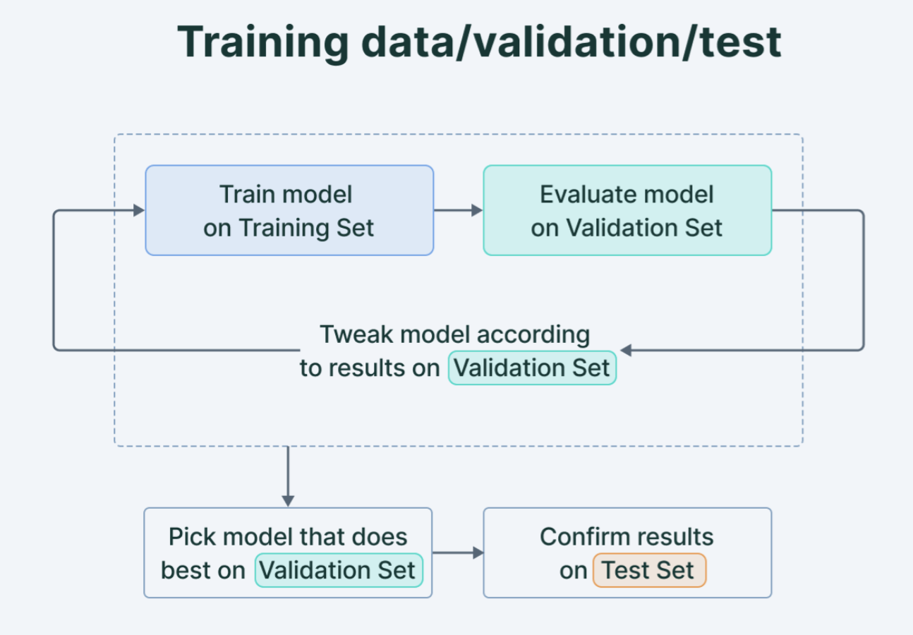
Train, Validate, Test!

Image Credit - Animesh Agarwal

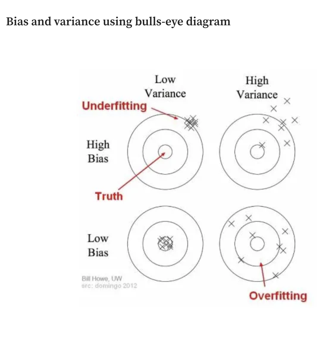
The Bias/Variance Tradeoff

\[ E[Y - (\widehat{Y}|X)] = \text{Var}(Y|X) + \text{Bias}(\widehat{Y}|X)^{2} + \text{Var}(\epsilon) \]

• \(\text{Var}(Y|X)\) - How much do our estimates for Y vary over a different training set X

  • High Variance is a symptom of overfitting

• \(\text{Bias}(\widehat{Y}|X)^{2}\) - The difference between the average prediction of our model and the correct value

  • High Bias is a symptom of underfitting

\(\text{Var}(\epsilon)\) - irreducible error (the noise in the data)

Graphically

Evidence of Overfitting

Workflow

Splitting your data

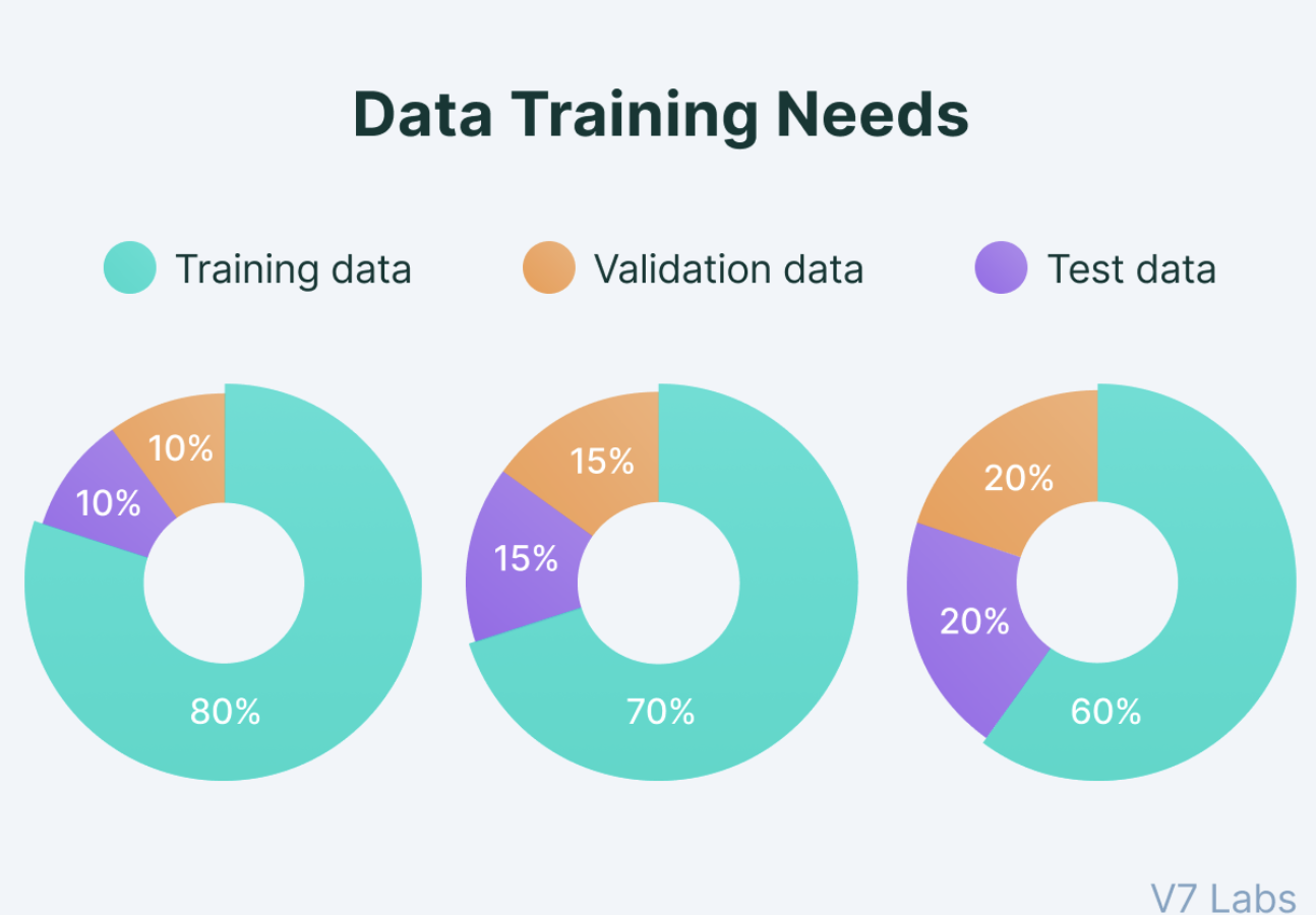
No optimal split, there are tradeoffs! 80/10/10 is most common. Or, as we will see, K-fold cross validation is an option!

The Most important rule

Never, Ever, Ever, Ever, Ever train expose your model to your test data!

This will lead to overfitting! It means your model is worthless! If you see crazy high accuracy, make sure your test data hasn’t leaked in.

Varieties of Classification

Don’t worry, you don’t have to read about European welfare states and corporatism. But there are many varieties of classification, we will cover only a few.

You already know how to classify!

What is this???

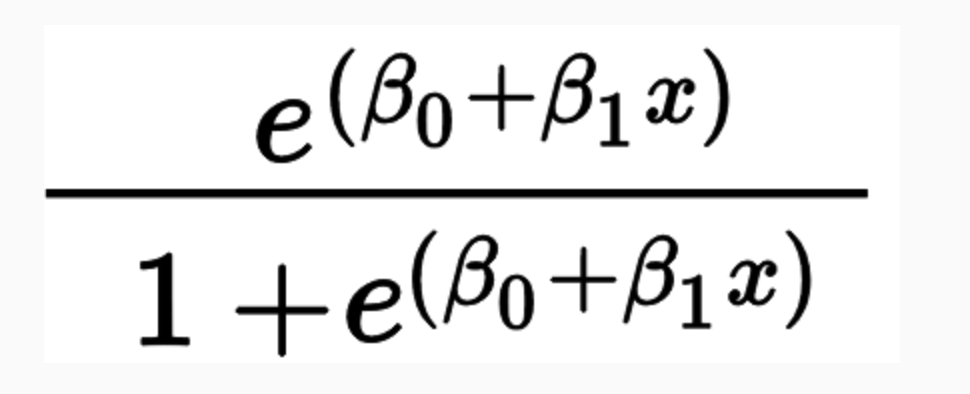
Logit!

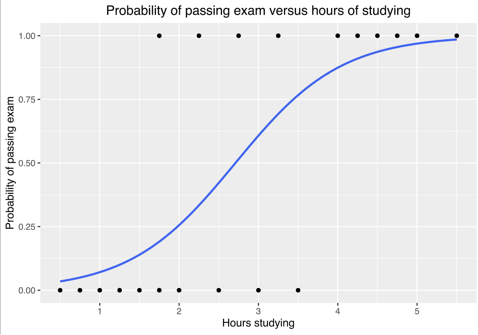
What is logit doing?

Logit models the probability that Y belongs to a particular category, given X.

\[ Pr(\text{Party = R |X = Death Tax}) \]

For a simple classification, if Pr(Party = R) > 0.5, we classify the speaker as a Republican.

The only difference from the logistic regression you learned in MLE is the workflow

The Gold Standard

The classifier which minimizes test error would be one that assigns each observation to it’s most likely class, given the observed data.

\[ \text{MAX:} Pr(Y = j| X= x) \]

Then, the (irreducible) error rate would be:

\[ 1 - E[\text{MAX:} Pr(Y = j| X= x)] \]

Why don’t we just do this????

A very simple classifier

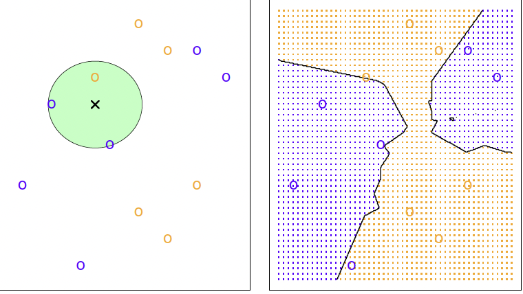
KNN with K = 3

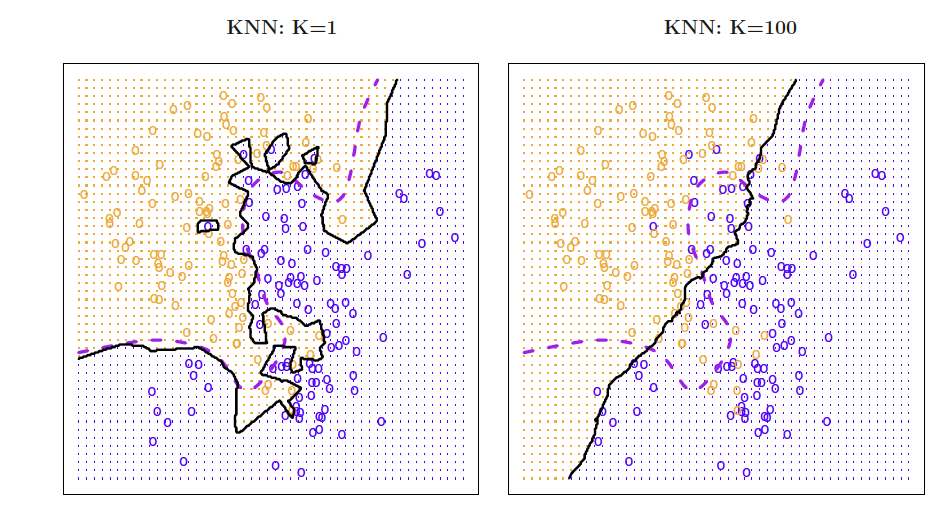
Overfitting and Underfitting

Validation

• We seek to minimize our test set error, but we train the data on a training set

  • So - how can we do it

• If we just select the model that performs best on the training data, we will almost certainly over fit!

• Solution: Create a separate validation set, evaluate training performance on validation rather than training set

Validation Drawbacks

• If the validation set is small, validation error can be highly valuable and poorly predictive of performance on test set

• But…if validation set is large, our model is trained on less data. The less data it’s trained on, the worse it will perform.

• Cross-Validation is a method that addresses these problems by leveraging the full training set while reducing the variance of validation metrics

Leave-one out cross validation

Metric

\[ \widehat{\text{CVError}}_{n} = \frac{1}{n} \sum_{i = 1}^{n} MSE_{i} \]

In words, the average sum of the squared errors for each observation

Advantages: Lower Bias and makes use of the full data so not sensitive to different validation splits

Issues with LOOCV

To run leave-one out, we have to fit the model n times.

If we are running a simple model, this is not a major concern. But for more complex models with non-linearities or very large data, this is a big issues.

Solution: K-Fold cross validiation

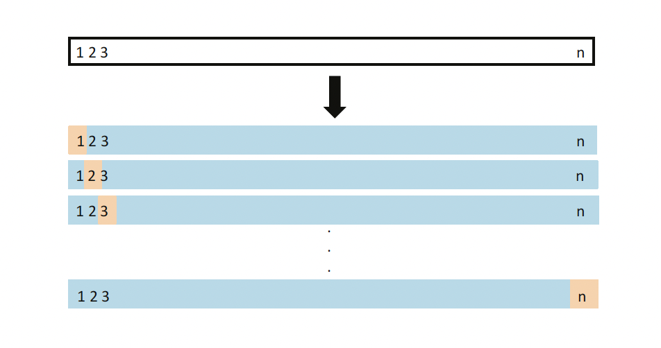
K-Fold Cross Validation

Split your training data into K folds.

Treat your first fold as the validation set.

Train the model on the other K-1 folds.

Repeat for each fold, using all other folds to train the model.

What is the relationship with LOOCV?

Why Prefer K-Fold?

In practice, K-Fold cross validation is very popular, and LOOCV is infrequently used. This is not only because of computational considerations.

Think back to the bias-variance trade off. LOOCV is fit on n-1 observations, which reduces bias. But it does this at a cost!

LOOCV fits n models with only one data different between each model. Each model is thus highly correlated. K-Fold models are less correlated with each other, as the training sets are more varied.

In Practice, we usually use K = 5 or k = 10 cross validation.

Bayes Theorem

Let \(\pi_{k}\) represent the probability that an observation comes from class k. Let \(f_{k}(x)\) denote the density function of X for an observation that comes from k. \((f_{k}(X) = \text{Pr}(X| Y= k)\)

Then, Bayes tells us:

\[ Pr(Y = k|X=x) = \frac{\pi_{k}f_{k}(x)}{\sum_{l=1}^{K}\pi_{l}f_{l}(x)} \]

We can estimate \(\pi_{k}\) easily; fraction of training observatios in each class. Getting \(f_{k}(x)\) is harder!

Naive Bayes

Let’s make a heroic assumption!

Assume that within each class k, the p predictors are independent.

If we do this, we can ignore the joint distributions of each predictor.

Is this believable? Almost never! ):

But…..it’s useful! (:

Some math

If the predictions are independent, then \[f_{k}(x) = f_{k1}(x_{1}) * f_{k2}(x_{2}) * f_{k3}(x_{3}) * ... * f_{kp}(x_{p}) \]

therefore

\[ Pr(Y = k|X =x) = \frac{\pi_{k}f_{k1}(x_{1}) * f_{k2}(x_{2}) * f_{k3}(x_{3}) * ... * f_{kp}(x_{p})}{\sum_{l = 1}^{K} \pi_{l} f_{k1}(x_{1}) * f_{k2}(x_{2}) * f_{k3}(x_{3}) * ... * f_{kp}(x_{p})} \]

Where we can estimate \(f_{k}(x)\) from the training data.

Naive Bayes Classification Example

Rows: 117,214
Columns: 18
$ date_received                <date> 2019-09-24, 2019-10-25, 2019-11-08, 2019…
$ product                      <chr> "Debt collection", "Credit reporting, cre…
$ sub_product                  <chr> "I do not know", "Credit reporting", "I d…
$ issue                        <chr> "Attempts to collect debt not owed", "Inc…
$ sub_issue                    <chr> "Debt is not yours", "Information belongs…
$ consumer_complaint_narrative <chr> "transworld systems inc. \nis trying to c…
$ company_public_response      <chr> NA, "Company has responded to the consume…
$ company                      <chr> "TRANSWORLD SYSTEMS INC", "TRANSUNION INT…
$ state                        <chr> "FL", "CA", "NC", "RI", "FL", "TX", "SC",…
$ zip_code                     <chr> "335XX", "937XX", "275XX", "029XX", "333X…
$ tags                         <chr> NA, NA, NA, NA, NA, NA, NA, NA, NA, NA, N…
$ consumer_consent_provided    <chr> "Consent provided", "Consent provided", "…
$ submitted_via                <chr> "Web", "Web", "Web", "Web", "Web", "Web",…
$ date_sent_to_company         <date> 2019-09-24, 2019-10-25, 2019-11-08, 2019…
$ company_response_to_consumer <chr> "Closed with explanation", "Closed with e…
$ timely_response              <chr> "Yes", "Yes", "Yes", "Yes", "Yes", "Yes",…
$ consumer_disputed            <chr> "N/A", "N/A", "N/A", "N/A", "N/A", "N/A",…
$ complaint_id                 <dbl> 3384392, 3417821, 3433198, 3366475, 33853…

We will model product as a function of the complaint text

What does the text look like?

[1] "I was sold access to an event digitally, of which I have all the screenshots to detail the transactions, transferred the money and was provided with only a fake of a ticket. I have reported this to paypal and it was for the amount of {$21.00} including a {$1.00} fee from paypal. \n\nThis occured on XX/XX/2019, by paypal user who gave two accounts : 1 ) XXXX 2 ) XXXX XXXX"

[1] "Over the past 2 weeks, I have been receiving excessive amounts of telephone calls from the company listed in this complaint. The calls occur between XXXX XXXX and XXXX XXXX to my cell and at my job. The company does not have the right to harass me at work and I want this to stop. It is extremely distracting to be told 5 times a day that I have a call from this collection agency while at work."

[1] "I would like to request the suppression of the following items from my credit report, which are the result of my falling victim to identity theft. This information does not relate to [ transactions that I have made/accounts that I have opened ], as the attached supporting documentation can attest. As such, it should be blocked from appearing on my credit report pursuant to section 605B of the Fair Credit Reporting Act."

Personal data is redacted to XXXX strings. Money is in brackets.

What if we want to extract dollar amounts?

complaints$consumer_complaint_narrative %>%
  str_extract_all("\\{\\$[0-9\\.]*\\}") %>%
  compact() %>%
  head()

[[1]]
[1] "{$21.00}" "{$1.00}" 

[[2]]
[1] "{$2300.00}"

[[3]]
[1] "{$200.00}"  "{$5000.00}" "{$5000.00}" "{$770.00}"  "{$800.00}" 
[6] "{$5000.00}"

[[4]]
[1] "{$15000.00}" "{$11000.00}" "{$420.00}"   "{$15000.00}"

[[5]]
[1] "{$0.00}" "{$0.00}" "{$0.00}" "{$0.00}"

[[6]]
[1] "{$650.00}"

Label and Split the Data

library(tidymodels)

set.seed(1234)
complaints2class <- complaints %>%
  mutate(product = factor(if_else(
    product == paste("Credit reporting, credit repair services,",
                     "or other personal consumer reports"),
    "Credit", "Other"
  )))

complaints_split <- initial_split(complaints2class, strata = product)

complaints_train <- training(complaints_split)
complaints_test <- testing(complaints_split)

dim(complaints_train)

[1] 87910    18

dim(complaints_test)

[1] 29304    18

One way to pre-processes

library(textrecipes)

complaints_rec <-
  recipe(product ~ consumer_complaint_narrative, data = complaints_train)

complaints_rec <- complaints_rec %>%
  step_tokenize(consumer_complaint_narrative) %>%
  step_tokenfilter(consumer_complaint_narrative, max_tokens = 1e3) %>%
  step_tfidf(consumer_complaint_narrative)

complaint_wf <- workflow() %>%
  add_recipe(complaints_rec)

The idea is that you create a recipe which you can then apply to your test data as well to ensure equivalent preprocessing without leakage.

Set up the model

library(discrim)
nb_spec <- naive_Bayes() %>%
  set_mode("classification") %>%
  set_engine("naivebayes")

nb_spec

Naive Bayes Model Specification (classification)

Computational engine: naivebayes 

K-Fold Cross Validate

set.seed(234)
complaints_folds <- vfold_cv(complaints_train)

Default is 10 folds, so a 90/10 split

nb_wf <- workflow() %>%
  add_recipe(complaints_rec) %>%
  add_model(nb_spec)

nb_rs <- fit_resamples(
  nb_wf,
  complaints_folds,
  control = control_resamples(save_pred = TRUE)
)

Performance (1)

nb_rs_metrics <- collect_metrics(nb_rs)
nb_rs_predictions <- collect_predictions(nb_rs)

nb_rs_metrics

# A tibble: 2 × 6
  .metric  .estimator  mean     n std_err .config             
  <chr>    <chr>      <dbl> <int>   <dbl> <chr>               
1 accuracy binary     0.807    10 0.00464 Preprocessor1_Model1
2 roc_auc  binary     0.883    10 0.00173 Preprocessor1_Model1

ROC Curve

Confusion Matrix

Can we calculate precision and recall?

Comparing to a baseline

null_classification <- null_model() %>%
  set_engine("parsnip") %>%
  set_mode("classification")

null_rs <- workflow() %>%
  add_recipe(complaints_rec) %>%
  add_model(null_classification) %>%
  fit_resamples(
    complaints_folds
  )

null_rs %>%
  collect_metrics()

# A tibble: 2 × 6
  .metric  .estimator  mean     n std_err .config             
  <chr>    <chr>      <dbl> <int>   <dbl> <chr>               
1 accuracy binary     0.526    10 0.00143 Preprocessor1_Model1
2 roc_auc  binary     0.5      10 0       Preprocessor1_Model1

Regularization

We have a ton (1000) of features doing the predicting here! Many of these features are poor predictors; a simpler model may generalize better to new data.

We do this by applying a penalty to extra features, which then shrinks coefficients close to zero unless they are highly predictive.

Popular approaches are Ridge, Lasso, and Elastic Net

Ridge

Recall that OLS is minimizing

\[ \sum_{(x,y)\in D} (y - \text{prediction(x)})^{2} \]

With Ridge, we minimize a slightly different function, where we add a penalty

\[ \sum_{(x,y)\in D} (y - \text{prediction(x)})^{2} + \lambda\sum\beta_{j}^{2} \]

where \(\lambda\) is a hyperparameter set by the user

Ridge Penalty Term

\[ \lambda\sum\beta_{j}^{2} \]

This will be small either when \(\lambda\) is closer to 0, or when \(\beta\) is close to 0. The higher \(\lambda\), the quicker the coefficients shrink towards 0.

In practice, we tune the parameter. Often, we use a technique called grid search.

Note that we don’t shrink \(\beta_{0}\) because the intercept is simply a measure of the mean value of the response when all the x = 0.

Why does it work?

We know that OLS is BLUE. Here we are introducing bias through the penalty term.

But…recall that \[ E[Y - (\widehat{Y}|X)] = \text{Var}(Y|X) + \text{Bias}(\widehat{Y}|X)^{2} + \text{Var}(\epsilon) \]

In datasets with many variables, OLS estimates will have high variance, and if features > observations, OLS cannot be fit whereas Ridge will still produce good estimates.

Lasso

Ridge will include all p predictors in the final model, but unless \(\lambda = \infty\) it will not set coefficients to zero.

We might want to just include the most predictive features (for better prediction or for parsimony).

\[ \sum_{(x,y)\in D} (y - \text{prediction(x)})^{2} + \lambda\sum |{\beta_{j}}|\]

Alternatively, we can say that Lasso applies an \(\ell_{1}\) penalty and Ridge applies an \(\ell_{2}\) penalty

An Alternative Formulation

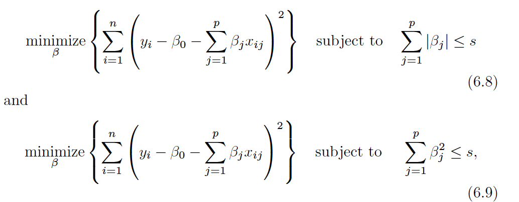
where \(\lambda\) determines s. The larger s (the lower \(\lambda\)) the closer to OLS we are

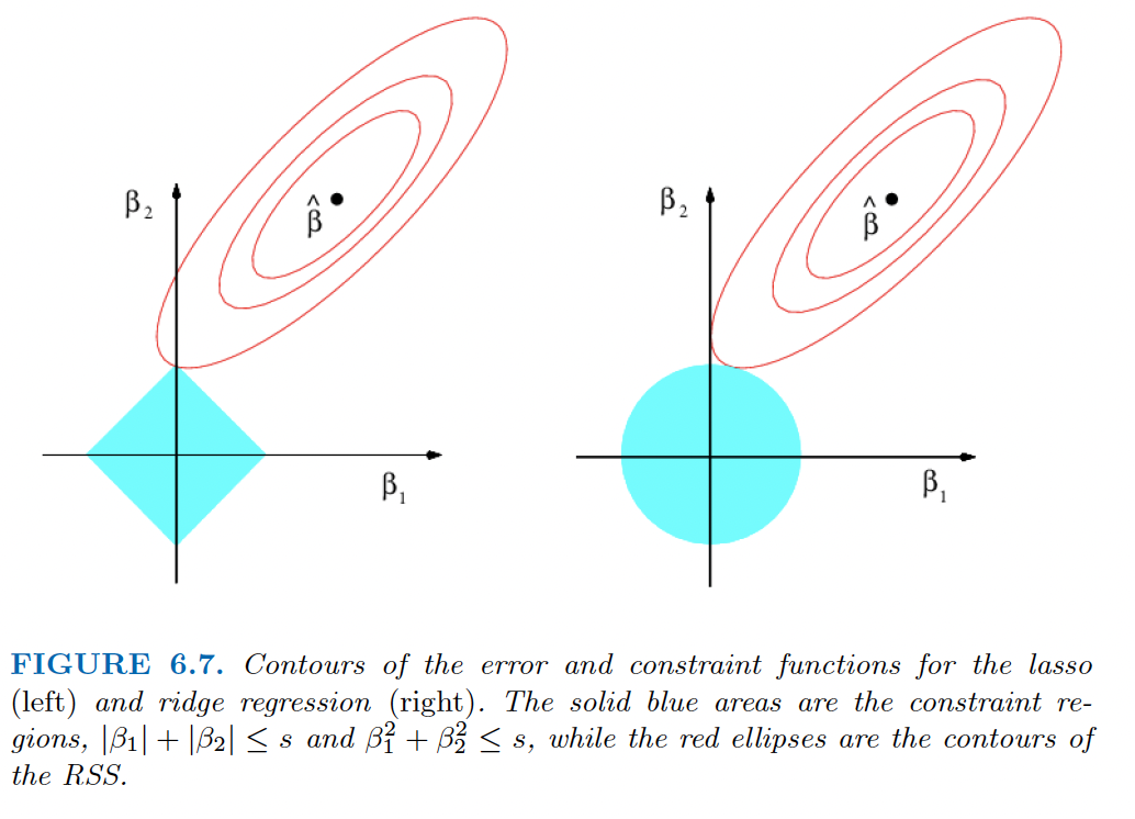
We can see that the shape of the lasso allows constraint for coefficients to be set to zero.

Which is better?

• If we have reason to believe that many variables are truly non-predictive, Lasso works well

• If none or few of the true \(\beta\) are zero, Ridge works better

• Neither universally dominates

  • so try both!

• Elastic Net is an alternative approach that is a linear combination of the two

An Aside

Review

• Why do we train - validate - test?

• What is the goal of regularization methods like Lasso and Ridge?

• What is the difference between the two?

• What is a hyperparamter?

Implementation

We can apply the penalty to logistic regression (for classification) as well. Again I adapt Silge and Hvitfeldt, because the tidymodels package is a user friendly approach to fitting ML models.

lasso_spec <- logistic_reg(penalty = 0.01, mixture = 1) %>%
  set_mode("classification") %>%
  set_engine("glmnet")

mixture = 1 specifies that this a logit, where we’ve set the penalty to be .001

mixture = 0 would specify a ridge and a value between 0 and 1 would specify an elastic net

Again we use K-fold CV

set.seed(30307)

lasso_rs <- fit_resamples(
  lasso_wf,
  complaints_folds,
  control = control_resamples(save_pred = TRUE)
)
lasso_rs_metrics <- collect_metrics(lasso_rs)
lasso_rs_predictions <- collect_predictions(lasso_rs)

lasso_rs_metrics

# A tibble: 2 × 6
  .metric  .estimator  mean     n  std_err .config             
  <chr>    <chr>      <dbl> <int>    <dbl> <chr>               
1 accuracy binary     0.870    10 0.00126  Preprocessor1_Model1
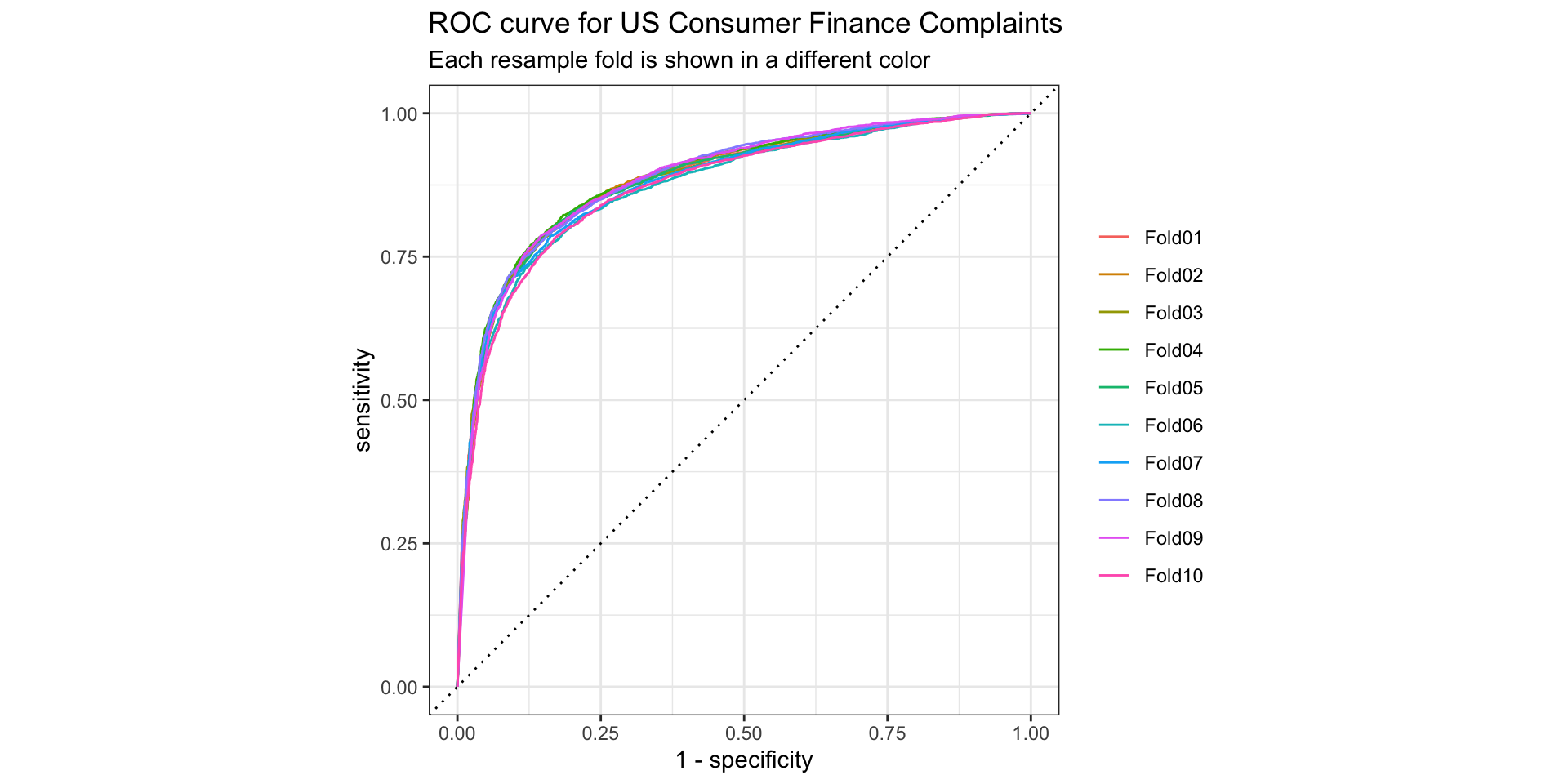
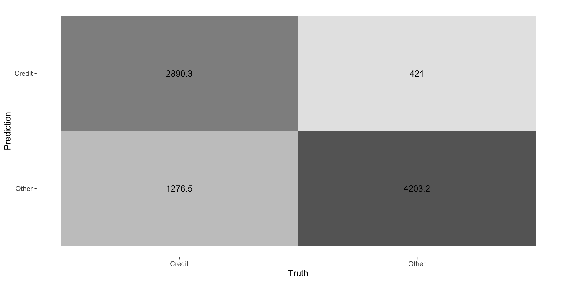
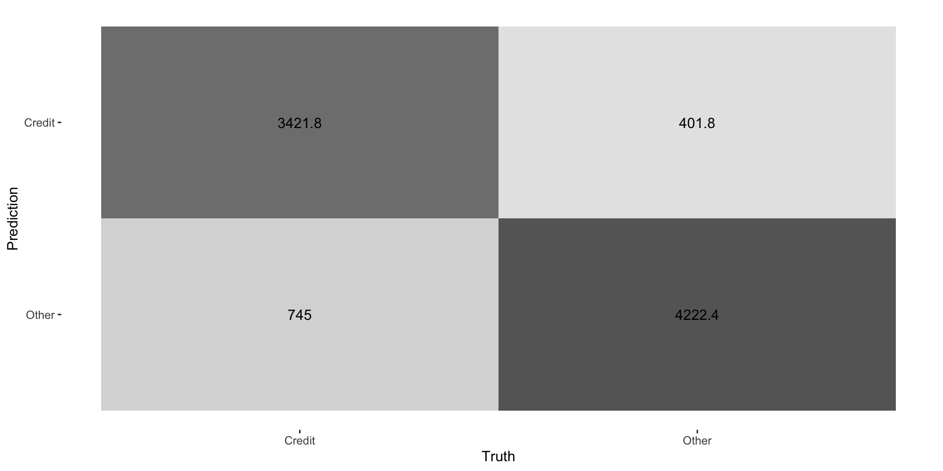
2 roc_auc  binary     0.939    10 0.000641 Preprocessor1_Model1

ROC Curve

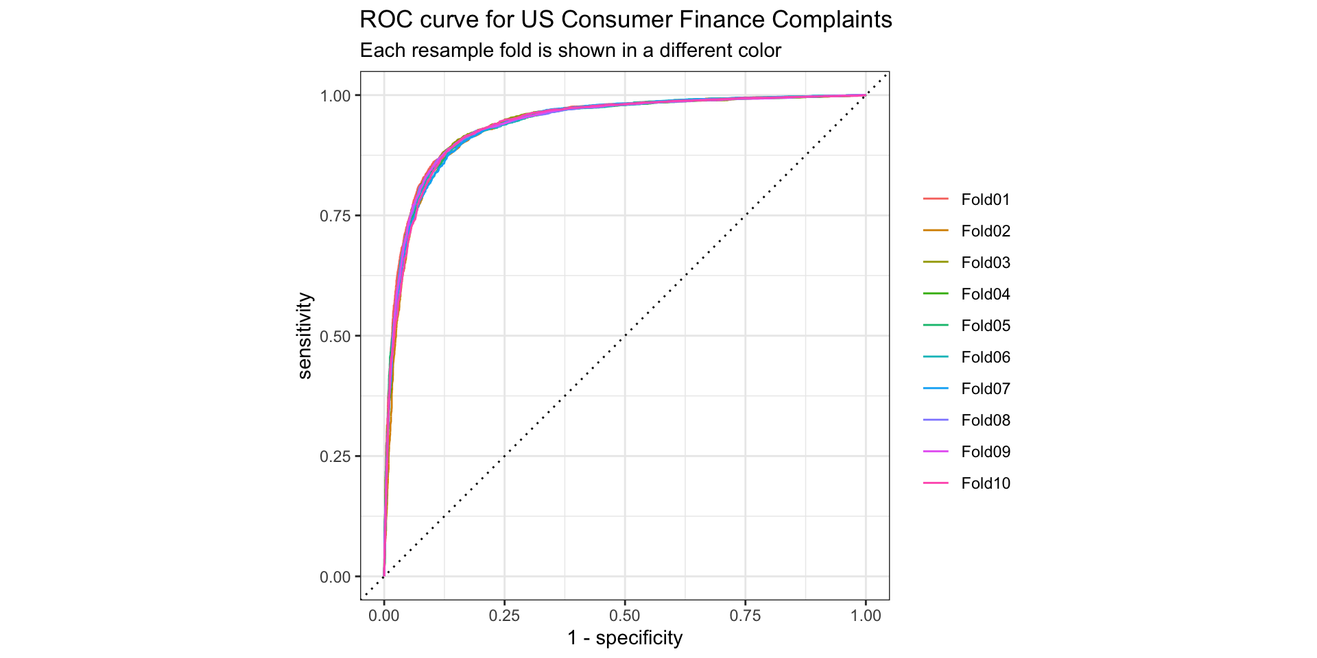
Confusion Matrix

Hyperparameter Tuning

We set \(\lambda\) to .01. This was arbitrary! We can (probably) do better.

tune_spec <- logistic_reg(penalty = tune(), mixture = 1) %>%
  set_mode("classification") %>%
  set_engine("glmnet")
## now we have a placeholder for penalty
lambda_grid <- grid_regular(penalty(), levels = 30)
## grid_regular will select 30 possible values for the penalty
lambda_grid

# A tibble: 30 × 1
    penalty
      <dbl>
 1 1   e-10
 2 2.21e-10
 3 4.89e-10
 4 1.08e- 9
 5 2.40e- 9
 6 5.30e- 9
 7 1.17e- 8
 8 2.59e- 8
 9 5.74e- 8
10 1.27e- 7
# ℹ 20 more rows

Run the model over the grid

tune_wf <- workflow() %>%
  add_recipe(complaints_rec) %>%
  add_model(tune_spec)

set.seed(30307)
tune_rs <- tune_grid(
  tune_wf,
  complaints_folds,
  grid = lambda_grid,
  control = control_resamples(save_pred = TRUE)
)

Note - this can take some time because we have to fit a bunch of models!

Select the best model

tune_rs %>%
  show_best("roc_auc")

# A tibble: 5 × 7
       penalty .metric .estimator  mean     n  std_err .config              
         <dbl> <chr>   <chr>      <dbl> <int>    <dbl> <chr>                
1 0.000788     roc_auc binary     0.953    10 0.000502 Preprocessor1_Model21
2 0.000356     roc_auc binary     0.953    10 0.000504 Preprocessor1_Model20
3 0.000161     roc_auc binary     0.953    10 0.000511 Preprocessor1_Model19
4 0.0000728    roc_auc binary     0.953    10 0.000516 Preprocessor1_Model18
5 0.0000000001 roc_auc binary     0.953    10 0.000517 Preprocessor1_Model01

chosen_auc <- tune_rs %>%
  select_best(metric = "roc_auc", -penalty)

chosen_auc

# A tibble: 1 × 2
   penalty .config              
     <dbl> <chr>                
1 0.000788 Preprocessor1_Model21

Note - depending on application we could select a different metric, like accuracy or precision or F1 score.

Fit the chosen mode and explore the data

final_lasso <- finalize_workflow(tune_wf, chosen_auc)

fitted_lasso <- fit(final_lasso, complaints_train)

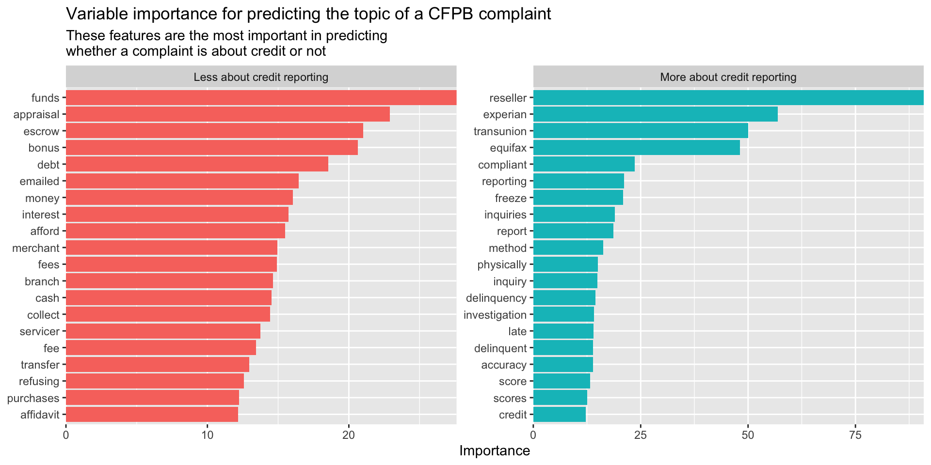
Let’s do a sanity check to see if sensible words predict credit reporting as the category

fitted_lasso %>%
  extract_fit_parsnip() %>%
  tidy() %>%
  arrange(estimate)

# A tibble: 1,001 × 3
   term                                          estimate  penalty
   <chr>                                            <dbl>    <dbl>
 1 tfidf_consumer_complaint_narrative_reseller      -90.9 0.000788
 2 tfidf_consumer_complaint_narrative_experian      -56.9 0.000788
 3 tfidf_consumer_complaint_narrative_transunion    -50.1 0.000788
 4 tfidf_consumer_complaint_narrative_equifax       -48.1 0.000788
 5 tfidf_consumer_complaint_narrative_compliant     -23.7 0.000788
 6 tfidf_consumer_complaint_narrative_reporting     -21.1 0.000788
 7 tfidf_consumer_complaint_narrative_freeze        -20.9 0.000788
 8 tfidf_consumer_complaint_narrative_inquiries     -19.0 0.000788
 9 tfidf_consumer_complaint_narrative_report        -18.6 0.000788
10 tfidf_consumer_complaint_narrative_method        -16.3 0.000788
# ℹ 991 more rows

Final Fit: Use the test data

final_fitted <- last_fit(final_lasso, complaints_split)

collect_metrics(final_fitted)

# A tibble: 2 × 4
  .metric  .estimator .estimate .config             
  <chr>    <chr>          <dbl> <chr>               
1 accuracy binary         0.891 Preprocessor1_Model1
2 roc_auc  binary         0.954 Preprocessor1_Model1

Note that the final model has a near identical area under curve and accuracy (we could/should compute other metrics too) - this means we didn’t overfit!

Feature Importance

Note - I can share the .qmd file if you want code for any of the above.

Tree Based Models

• Tree Based models have a very different logic than logit and naive bayes.

  • Segment the decision space into regions based on decision trees

  • Very good at handling non-linearity

• Simple decision try methods are easy to interpret and intuitive, but performance is not that great

• Random forests are more complex and tend to perform very well

Decision Trees are Intuitive!

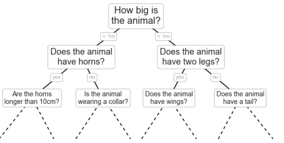
Terminology

Node: each subset created by a split

Leaf or Terminal Node: The final subsets of the data

Root: The top of the tree (first note/unsplit data)

Depth: How many layers of Nodes there are

Visualizing Depth

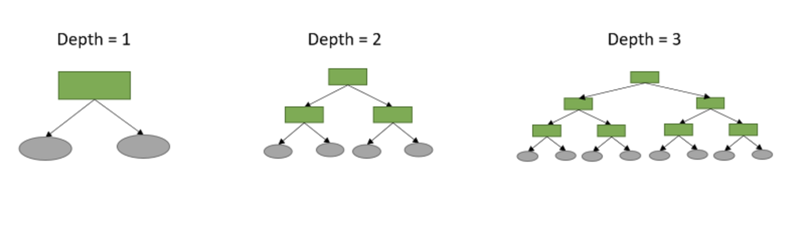
Trees are often substantially deeper, but there is a tradeoff between depth and interpretability.

A Simple Regression Tree

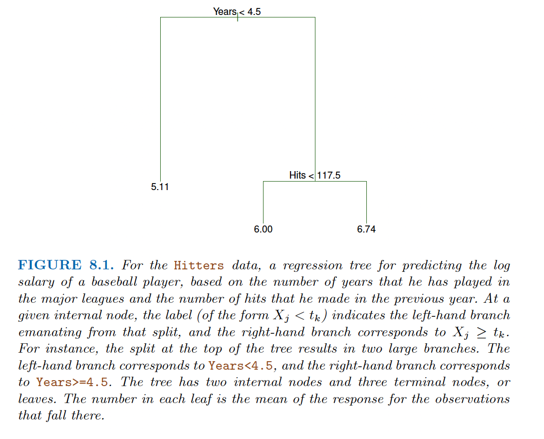
Each leaf is a prediction based on the mean value within that subset. For example, we see that the average \(log_{10}\) of salary is 5.11 ($165,165) for players who have played less than 4.5 years.

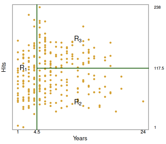
Corresponding Data Partition

More complex partitions

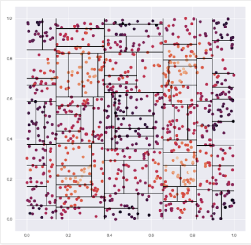
A moderately complex partition predicting a highly non-linear relationship

Regression Tree Recipe

• Divide the feature (or predictor) space (all possible values of the X variables) into J distinct and non-overlapping regions

  • This should remind you of clustering!

• For each partition, we assign the mean of the Y value(s) to each observation in the partition

  • This should remind you of how the cluster centers are updated!

• But…….how do we decide how to partition the data?

Goal of splitting

We hope to minimize the following objective function:

\[ \sum_{j =1}^{J}\sum_{i\in R_{j}} (y_{i} - \widehat{y}_{R_{j}})^{2} \]

This should look (kinda) familiar! What are we minimizing?

Recursive Binary Splitting

Minimzing the objective function by considering all splits is computationally infeasible.

Instead, we use a top down, greedy approach called recursive binary splitting.

Top down - we start from the root of the tree and successively split as we descend

Greedy - we make the best split at the particular layer we are at, without looking down the tree

Intuition: We make the split that leads to the greatest reduction in RSS (the objective function).

Mathematically

Let \(R_{j}\)be a partition of the feature space for feature \(x_{j}\) and let s be a potential cutpoint

\[ R_{1}(j,s) = [X|X_{j} < s] \text{ and } R_{2}(j,s) = [X|X_{j} \geq s] \]

then we want to find the value of j and s that minimize

\[ \sum_{i:x_{i}\in R_{1}(j,s)} (y_{i} - \widehat{y}_{R_{1}})^{2} \text{ and } \sum_{i:x_{i}\in R_{2}(j,s)} (y_{i} - \widehat{y}_{R_{2}})^{2} \]

Help me out! What are we minimizing?

When do we stop splitting?

Prior to beginning our process, we set a stop rule.

This could be a certain level of the Residual Sum of Squares

Or it could be that no split exists which improves the RSS by our desired valued

Or it could be that we stop once all partitions are of size less than N

These are also hyperparameters

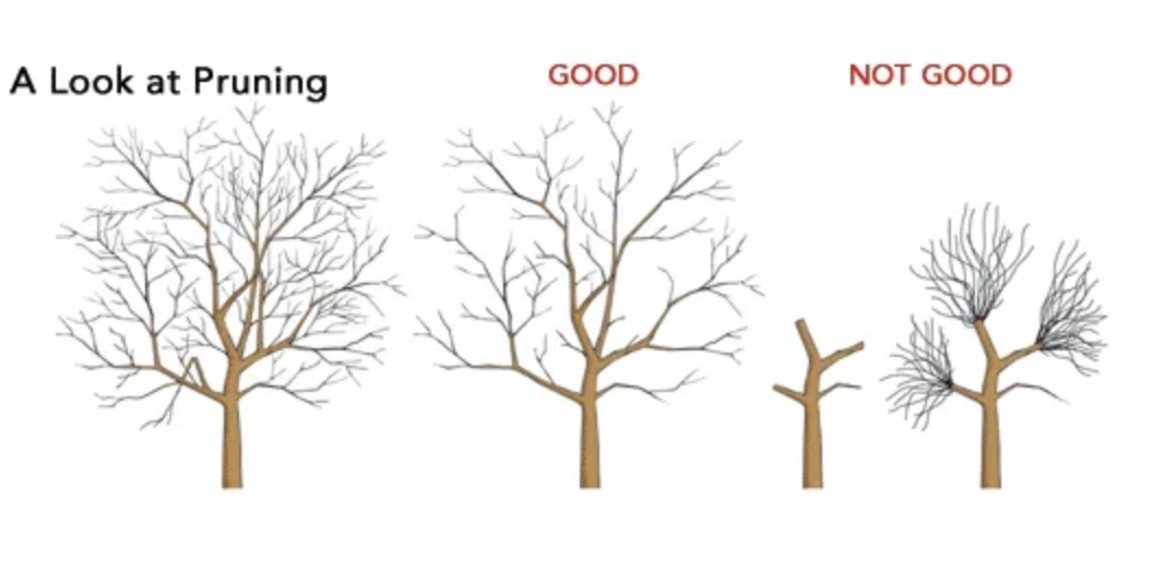
Pruning the Trees

Since tree based regressions set out to find complex non-linearities, they are prone to overfitting.

We set out to grow very simple trees, which are less likely to overfit. But these might lead to missing real patterns in the data.

Instead, we grow deep trees with lots of branches. Then we prune them by removing branches that don’t improve our test/validation error to create a subtree.

Once again, this is hard because there are many possible subtrees from even a moderately complex tree.

Pruning Goal

Intuition

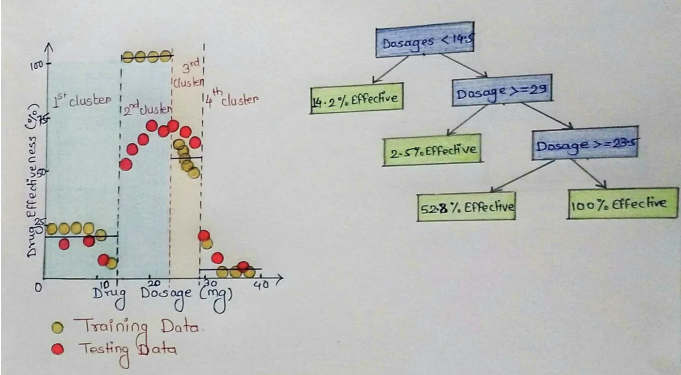
Image Credit - Sanchita Mangale

Intuition - New Subtree

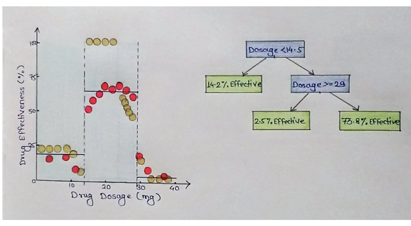
Image Credit - Sanchita Mangale

Cost Complexity Pruning

The intuition of cost complexity pruning is the same as regularization as in Ridge or Lasso.

Start at the bottom (leafs) of the tree, and consider removing a leaf. This creates a possible set of new subtrees.

Give each potential subtree a score:

\[ \text{Tree Score} = SSR + \alpha |T| \]

where T is the number of terminal nodes (leaves). For any \(\alpha\) there is an optimal subtree that minimizes the Tree Score.

We can use K-fold cross validation to find optimal trees.

Tree Based Classification

A slightly different objective function:

\[ \text{Classification Error Rate} = 1 - \sum_{i = 1}^{K}\frac{\text{Correctly Classified}}{\text{Total classified}} \]

For reasons beyond the scope of this course, minimizing Entropy or Gini performs better and is preferred:

\[ \text{Gini} = \sum_{k = 1}^{K}\widehat{p}_{mk}(1 - \widehat{p}_{mk}) \text { or } \text{Entropy} = - \sum_{k =1}^{K} \widehat{p}_{mk}log\widehat{p}_{mk} \]

From the trees to the forest

• Trees are interpetable, even for non-mathy people.

• They are fantastic at handling non-linearities

• However, the are highly unstable based on training data (display high varialnce)

• They are bad at handling truly linear relationships

• Accuracy may also be poor - unless we aggregate many decision trees to create a forest

Bagging

Analogous to bootstrapping (which may have been covered in OLS or MLE?)

Intuition: Our trees suffer from high variance. If we could train it on more data, we could decrease the variance.

Problem: We only have one training set.

Solution: We can bootstrap ourselves B new training sets from the initial training set and average predictions over them

Mathematically

Let f(x) be our model, which is a complete tree without pruning. Then we can use bagging to obtain:

\[ \widehat{f}_{bagging}(x) = \frac{1}{B}\sum_{b = 1}^{B} \widehat{f}_{b}(x) \]

For classification, rather than averaging we use plurality rules to select the class for each partition. A common hyperparamter setting is to use 100 bags.

Moreover, we can more cheaply estimate test error by using Out-of-bag error rather than using cross-validation.

From Bagged Trees to Random Forests

• In bagging, the trees that are generated are highly correlated, because they always consider the same set of splits over correlated sets of data

  • This makes our models inefficient

• Random Forests decorrelate the trees

• Each time a split is considered, the split is only considered over a random sample of predictors

  • Why does this work?

• An important Random Forest hyperparameter is m, the number of predictors considered at each split.

TL;DR and extensions

• By aggregating across many trees bagging improves on single tree based methods

• Random Forest improves accuracy further (to near state-of-the-art levels) by decorrelating the trees

• Further refinements exist including:

  • Boosting: Learns sequentially using information from the previously fit trees

    • has many sub-flavors

  • BART: Bayesian approach, where we draw new trees from the posterior distribution

Support Vector Machines

• Cavaet: A speed run through SVM so that we can give adequate attention to Deep Learning and transformers

• Intuiton: We are searching for the optimal hyperplane to separate our data.

  • A hyperplane in p-dimensional space is a subspace of dimension p-1.

  • For example, in a two dimensional space it’s a line. In three dimensional space, it’s a plane (think a piece of paper)

  • What we want to do is find the hyperplane (in two dimensions line) that best splits the data

How do we define a hyperplane

In two dimensions, a hyperplane (line) is defined as:

\[ 0 = \beta_{0} + \beta_{1}X_{1} \]

In three dimensions, a hyperplane (plane) is defined as:

\[ 0 = \beta_{0} + \beta{1}X_{1} + \beta_{2}X_{2} \]

So, can we use inductive reasoning to figure out a general formula?

Separating Hyperplanes

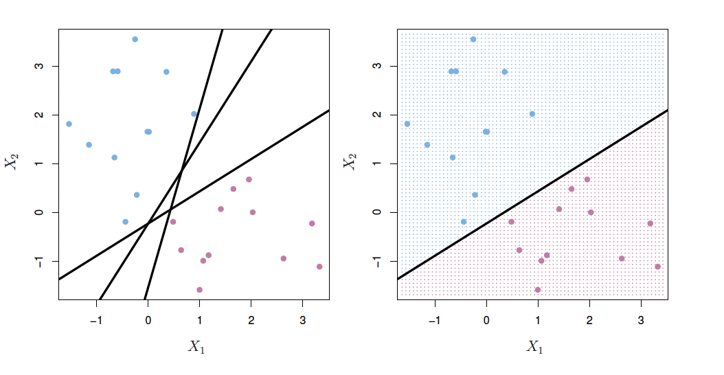
So - we assign class based on which side of the hyperplane the data is on. And we can measure confidence based on euclidean distance of predicted value from hyperplane

The Best Hyerplane

If our data can be perfectly split by a hyperplane, it can be perfectly split by an infinite number of hyperplanes.

Then, the best hyperplane, aka the maximal margin classifier, is the hyperplane which lies furthest away from the training observations.

WHY?

The Support of the Hyperplane

The support of the hyperplane are the points for which the maximal margin hyperplane would shift were those points to shift.

A problem

Usually, unless the data is very friendly and highly linear, we cannot construct a seperating hyperplane.

But… we can construction an almost separating hyerplane instead.

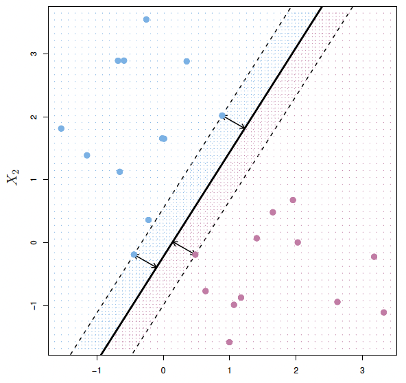
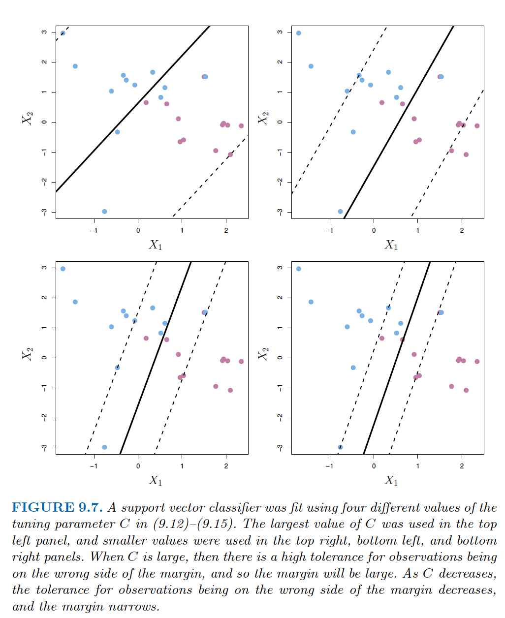
We construct a hyperplane, but allow for some misclassification (where there is a hyperparameter C which determines sensitivity to hyperplane violations).

Specifically, the more forgiving our hyperparamter the less we overfit at the cost of introducing bias. The tradeoff strikes again!

Support Vector Machines with Different C

SML TL;DR

• Train, Validate, Test

• Cross Validation often an efficient method for training

• Know what hyperparameters to tune for each class of model

• No universally best model

• There is always a bias/variance tradeoff